Import the datasets into R

## Data for mapping:
load('fake-dorado-map-data.RData', verbose=TRUE)

## Loading objects:
##   fake.dorado

head(fake.dorado)

##   Year latitude longitude flag_id alb_mt bet_mt yft_mt
## 1 2015        4       191      JP   0.11   0.40   0.20
## 2 2015        4       192      JP   0.34   0.16   0.08
## 3 2015        4       193      JP   0.14   1.12   0.56
## 4 2015        4       194      JP   0.53   0.06   0.03
## 5 2015        4       195      JP   0.43   0.10   0.05
## 6 2015        4       196      JP   0.11   1.24   0.62

## EEZ Data
#eez overlay
eez        <- read.table("EZNEW2.txt", sep=" ", header=F, skip=0) #All regions
eez_pna  <- read.csv("pna_eez.csv") #PNA regions

## Import continent line dataset
load(file = 'continent-outlines-only.RData', verbose=TRUE)

## Loading objects:
##   countrydf

all_states <- map_data("world2Hires")

A very simple heatmap

subdo <- subset(fake.dorado, fake.dorado$Year == 2015)
# how many rows with each year in my original dataset
table(fake.dorado$Year) 

## 
## 2015 2016 
##  420  420

# how many rows in my filtered dataset
table(subdo$Year)

## 
## 2015 
##  420

table(subdo$flag_id)

## 
##  JP  TW 
## 210 210

# subset for JP only
subdo_jp <- subset(subdo, subdo$flag_id == 'JP')
table(subdo_jp$flag_id) 

## 
##  JP 
## 210

p <- ggplot() +
  geom_tile(data=subdo_jp, aes(x=longitude, y=latitude, fill=alb_mt))
p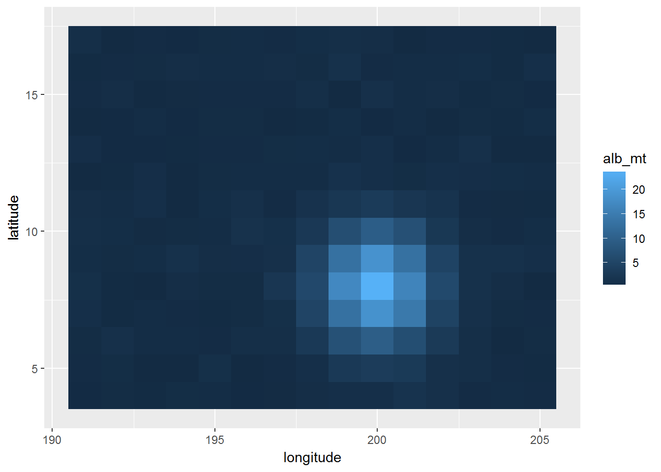

Make a heatmap of the yellowfin catch

p <- ggplot() +
  geom_tile(data=subdo_jp, aes(x=longitude, y=latitude, fill=yft_mt))
p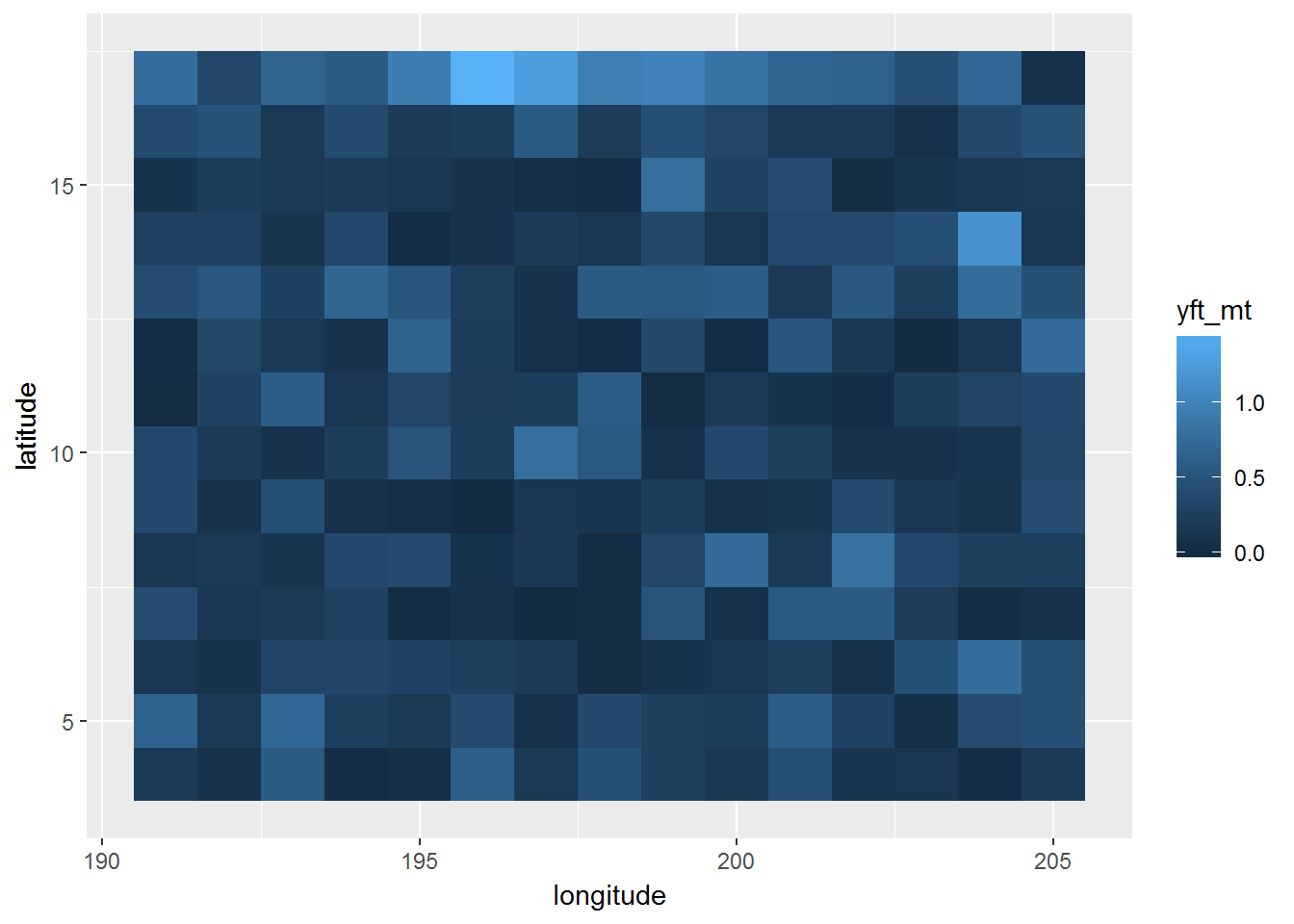

Make a heatmap of the bigeye catch

p <- ggplot() +
  geom_tile(data=subdo_jp, aes(x=longitude, y=latitude, fill=bet_mt))
p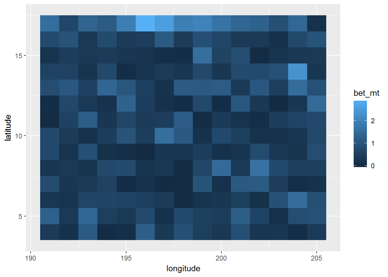

Make a heatmap with a different colour scheme:

p <- ggplot() +
  geom_tile(data=subdo_jp, aes(x=longitude, y=latitude, fill=alb_mt)) +
  scale_fill_distiller(palette = 'Spectral')
p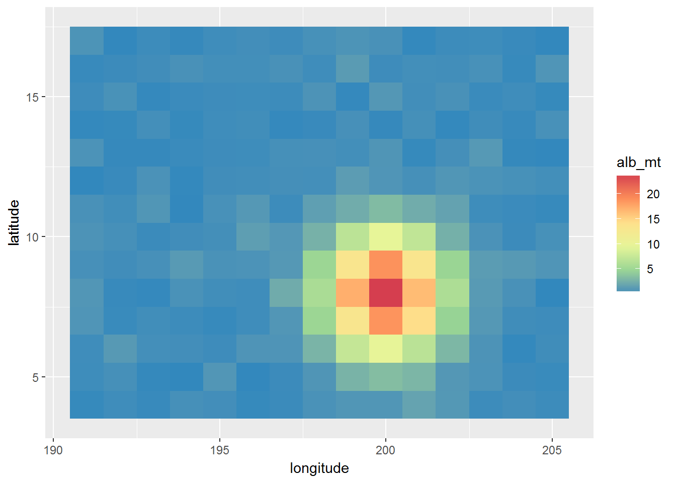

p <- ggplot() +
  geom_tile(data=subdo_jp, aes(x=longitude, y=latitude, fill=alb_mt)) +
  scale_fill_distiller(palette = 'YlOrRd')
p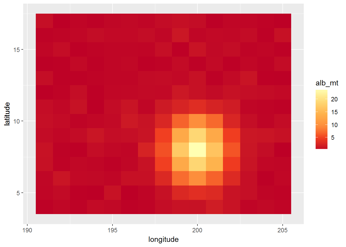

Now let’s add a new layer with EEZ outlines

p <- ggplot() +
  geom_tile(data=subdo_jp, aes(x=longitude, y=latitude, fill=alb_mt)) +
  scale_fill_distiller(palette = 'Spectral') +
  ## added a polygon layer with the EEZs, only drew EEZ outline (fill=NA)
  geom_polygon(data=eez, aes(eez[,1], eez[,2]), size=2, colour="white", fill=NA) +
  ## narrowed the x and y range of the plot to fit our dataset
  coord_cartesian(xlim=c(190,205), ylim=c(2,18)) +
  theme_bw() # make background white instead of grey
p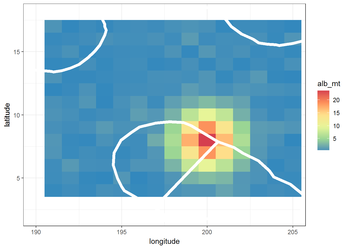

The next step is to add our continent layer:

p <- ggplot() +
  geom_tile(data=subdo_jp, aes(x=longitude, y=latitude, fill=alb_mt)) +
  scale_fill_distiller(palette = 'Spectral') +
  ## added a polygon layer with the EEZs, only drew EEZ outline (fill=NA)
  geom_polygon(data=eez, aes(eez[,1], eez[,2]), size=2, colour="white", fill=NA) +
  ## narrowed the x and y range of the plot to fit our dataset
  coord_cartesian(xlim=c(180,205), ylim=c(2,26)) +
  theme_bw() + # make background white instead of grey + 
  geom_path(data=countrydf, aes(x=lon, y=lat, group=id))
p

## Warning: Removed 53 rows containing missing values (geom_path).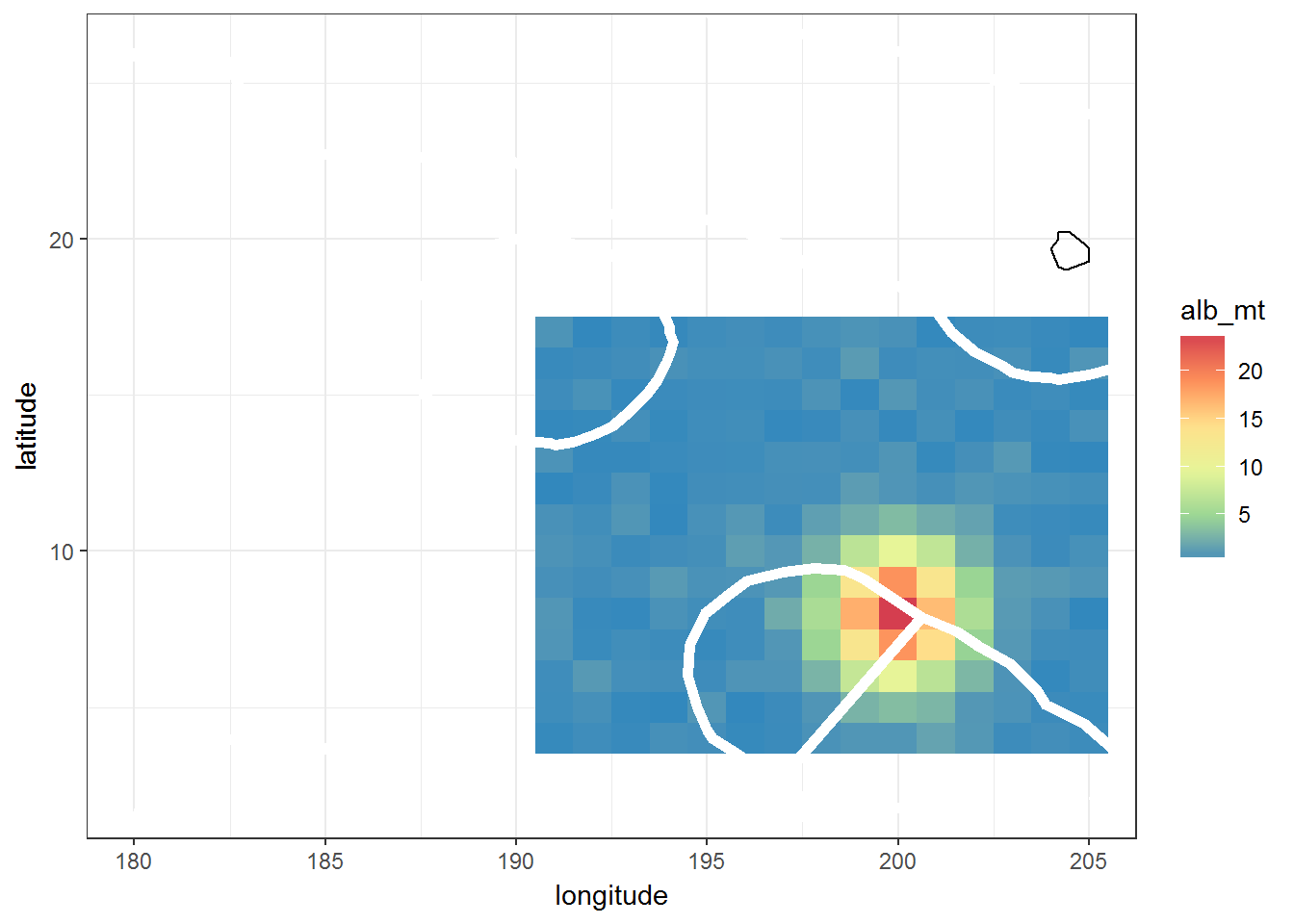

Draw this instead with the high resolution polygon dataset:

p <- ggplot() +
  geom_tile(data=subdo_jp, aes(x=longitude, y=latitude, fill=alb_mt)) +
  scale_fill_distiller(palette = 'Spectral') +
  ## added a polygon layer with the EEZs, only drew EEZ outline (fill=NA)
  geom_polygon(data=eez, aes(eez[,1], eez[,2]), size=2, colour="white", fill=NA) +
  ## narrowed the x and y range of the plot to fit our dataset
  coord_cartesian(xlim=c(180,205), ylim=c(2,26)) +
  theme_bw() + # make background white instead of grey + 
  geom_polygon(data=all_states, aes(x=long, y=lat, group = group),
               colour ="white",  fill="grey10" )
p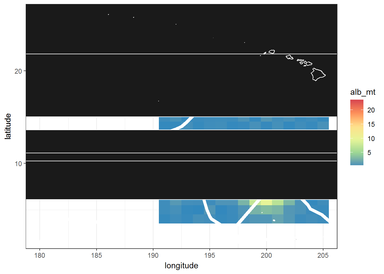

Making a map panel

p <- ggplot() +
  geom_tile(data=subdo, aes(x=longitude, y=latitude, fill=alb_mt)) +
  scale_fill_distiller(palette = 'Spectral') +
  ## added a polygon layer with the EEZs, only drew EEZ outline (fill=NA)
  geom_polygon(data=eez, aes(x=V1, y=V2), size=2, 
               colour="white", fill=NA) +
  ## narrowed the x and y range of the plot to fit our dataset
  coord_cartesian(xlim=c(190,205), ylim=c(2,19)) +
 # coord_equal() +
  theme_bw() +
  facet_wrap(~flag_id)
p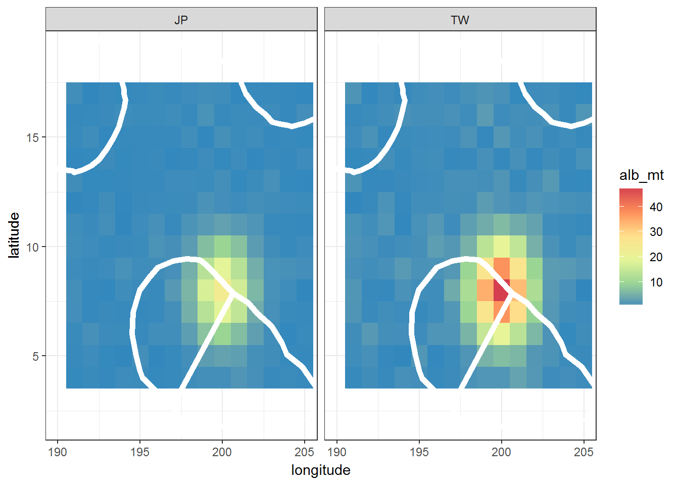

Exercises

Doing the same figure but with my Dorado extract. Make sure your Dorado folder (e.g. MH) in in the ggmaps folder. Note: for Dorado extracts only, need to specify fileEncoding='UTF-8-BOM'

dorado.dat <- read.csv('PW/PW custom report 100.csv', fileEncoding = 'UTF-8-BOM')